Assessing the Contribution of Glacier Melt to Discharge in the Tropics: The Case of Study of the Antisana Glacier 12 in Ecuador

1 Introduction

Tropical glaciers refer to ice bodies found at high elevations in a region where the diurnal temperature variations are more significant than the seasonal ones (Kaser and Osmaston, 2002). These glaciers are characterized by the occurrence of melting all year round because the 0°C isotherm remains continuously near the glacier fronts. Thus minimal energy inputs generate runoff (Francou et al., 2013). This aspect makes tropical glaciers suitable climatical indicators due to their quick mass balance response to temperature and precipitation variations (Ramírez et al., 2001; Francou et al., 2004). The Andes host 99% of tropical glaciers (Kaser and Osmaston, 2002), and they play an important role in the freshwater supply for cities located in the lowlands, especially during seasons with low or scarce precipitation (Chevallier et al., 2011; Buytaert et al., 2017).

Most precipitation in the eastern slopes of the Andes occurs due to dominant easterly winds which transport moisture from the Amazon basin and are forced to rise when encountering this barrier (Espinoza et al., 2020). Also, there is a contribution from the eastern Pacific, which triggers convection and precipitation over western slopes (Segura et al., 2019). These conditions ensure significant precipitation year-round in the Equatorial Andes. However, the rain-snow partitioning relies on temperature variability, conditioning the layer of snow on glaciers (Francou et al., 2004; Sagredo et al., 2014; Campozano et al., 2021), which in turn controls the surface albedo of the glacier (Favier et al., 2004b; Vincent et al., 2005).

Vuille et al. (2000, 2008) estimated that the Andes of Ecuador experienced a warming of 0.1°C per decade since 1950, whereas the projected warming during the 21st century is estimated between 4 and 5°C. To examine the glacier response to current weather and projected scenarios, a monitoring program was initiated in Ecuador by French Development Research Institute (IRD), Instituto Nacional de Meteorología e Hidrología (INAMHI) and Empresa Pública Metropolitana de Agua Potable y Saneamiento de Quito (EPMAPS) in June 1994. This network currently includes rain gauges, water-height gauges in rivers and automatic weather stations (AWS) installed at the ground level between 3,500 and 5,000 m a.s.l. but over different surface states, including paramo, moraine, and glacier surfaces (Villacís, 2008; Maisincho, 2015) around the Antisana Glacier 15 (AG15) (Francou et al., 2000; 2004). Initial results have shown the occurrence of an accelerated glacier retreat since the late 1970s (Cáceres et al., 2006; Rabatel et al., 2013). In addition, various Surface Energy Balance (SEB) modelings have been performed both at one point (Favier et al., 2004a) and at the scale of the entire glacier (Maisincho, 2015). Finally, another SEB modeling has been done over the snow-covered paramo using a coupled ground-snow model (e.g., ISBA/CROCUS, Wagnon et al., 2009).

These studies demonstrated that net short-wave radiation and albedo variations control melting rates in the ablation zone during most of the year. A melting minimum (compared to the mean observed melt during the rest of the year) was shown during the June-September season related to large energy losses associated with high sublimation rates. Likewise, the hydrological balance calculations showed that total glacier melting from AG15 are not directly drained into rivers at lower elevations, because significant amounts of water (>50%) are sunk before the glacier front, contributing to subsurface flows (Favier et al., 2008). The water drained from the watershed is even larger than previously calculated by Favier et al. (2008) because in their study he did not consider that the highest elevations of the glacier receive 60% more snow than the lowest slopes of the western flanks of the volcano (Basantes-Serrano et al., 2016). This increase was initially ignored in surface mass balance calculation on the AG15 (Francou et al., 2000; Francou et al., 2004) suggesting that the glacier-wide climatic balance values published before Basantes-Serrano et al. (2016) presented a significant negative bias.

To better assess the contribution of glaciers to lowland streamflow, the Antisana Glacier 12 (AG12) was monitored since 2004. Over this catchment, discharge modeling has only been done with conceptual and semi-empirical approaches (e.g., Villacís, 2008). The variations of melting with elevation and hence the origin of waters have never been clearly analyzed. This latter scientific concern is analyzed in this paper using a glacier-wide distributed SEB modeling and calculation of the transfer function of flows from each zone of the glacier towards the outlet of the catchment, which may result in more accurate results than statistical approaches (Veettil et al., 2017).

The distributed SEB has been successfully applied in many areas, but it requires a large amount of data to provide accurate results (Gerbaux et al., 2005; Hock and Holmgren, 2005; Anslow et al., 2008; Dadic et al., 2008; Naz et al., 2014; Ren et al., 2018). This glacier-wide modeling has been applied on the Zongo glacier in Bolivia (Sicart et al., 2011) and the Shallap glacier in Peru (Gurgiser et al., 2013a), demonstrating the crucial role of clouds in the longwave radiation budget and the role of solid precipitation in the net short-wave budget. However, these glaciers are not directly comparable to the Antisana Glaciers, which are located in an area with different climate settings (Favier et al., 2004b). The distributed SEB of AG15 has been investigated by Maisincho (2015) proving that the short-wave radiation and albedo exert first-order control on the energy available for melting on this glacier.

Here, we apply and validate this approach to demonstrate the processes that control the mass balance gradient and the corresponding discharge generated by melting at different altitudes. The amounts of melting in each altitude level were used as input for linear reservoirs and finally added to compute the simulated discharge (hereafter referred to as the potential discharge) that should be drained to the river downstream of the glacier if there were no underground losses.

The water discharge was computed over 23 months in 2011–2013. This spatialized computation allowed 1) investigating the variations of energy fluxes controlling the ablation and discharge production and 2) quantifying the water from different sources in the catchment. This paper is organized as follows: In Section 2 we describe the study site and the available data. The distributed SEB and the reservoir models are described in Section 3. In Section 4, we validate the coupled model and present results. In Section 5, we discuss the model uncertainties and the role of groundwater flow in AG12. Finally, our conclusions are presented in Section 6.

2 Study Site and Data

2.1 Study Site and Climate Settings

This study was conducted on the Glacier 12 (AG12) located in the “Los Crespos” catchment (2.9 km², 57% glacial cover) on the southwest flank of the Antisana volcano (Basantes-Serrano, 2015) in the Eastern Cordillera of Ecuador. AG12 spans from the summit at 5,720 m a.s.l. to glacier snout at 4,735 m a.s.l. covering a surface of 1.65 km², with a length of 2.3 km (Figure 1). The monthly temperature over the glacier snout remains homogeneous throughout the year at around 1.2°C on average (Figure 2). A slight temperature maximum is however observed between February-May (1.7°C) related to the period of higher humidity and cloudiness (Favier, 2004c); while the minimum between June-September (0.8°C) is related to the decrease in cloudiness and increase in wind speed. The 0°C isotherm shifts between 4,800 and −5,100 m a.s.l. (Basantes-Serrano et al., 2016) in accordance with the equilibrium line altitude (ELA) of the glacier around 5,030 m a.s.l. (Jomelli et al., 2009). Daily temperature variations exceed the seasonal ones, and this phenomenon is amplified by the radiative cooling and katabatic winds intensification during the night and early morning; which cause the temperature to drop below 0°C even at the glacier front (Favier et al., 2004b; Sklenár et al., 2015).

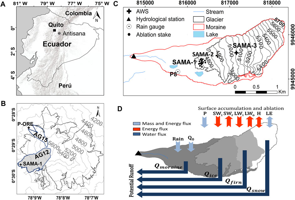
FIGURE 1. Study area: (A) Location of the Antisana volcano south-eastward of Quito, the capital of Ecuador. (B) Delineation of the studied glaciers in Antisana icecap: The Glacier 15 (AG15) on the northwest flank and the Glacier 12 (AG12) on the southwest shaded in gray. The location of the P-ORE and AWS SAMA-1 stations are also shown (black crosses). Cap outline and DEM taken from Basantes-Serrano (2015). (C) Distribution of monitoring network around Glacier 12 catchment. (D) Schema of processes simulated by the coupled glacier-hydrology model illustrating the fluxes of mass and energy between the atmosphere and land surface implemented over snow, glacier ice, and moraine. Arrows indicate P, precipitation; SWi, incident short-wave radiation; SWr, reflected short-wave radiation; LWi, downwelling longwave radiation; LWo, outgoing longwave radiation; H, sensible heat; and LE, latent heat. For moraine zone is also shown the Rain and basal ground flow Q₀.

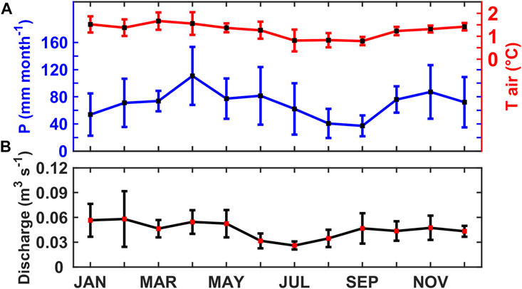
FIGURE 2. (A) Monthly precipitation values (blue line) measured at P8 rain gauge between 2005 and 2015, vertical bars represent monthly standard deviation. The same for air temperature (red line) measured at SAMA-1 between 2011 and 2015. (B) Mean monthly discharge measured (black line) in Los Crespos hydrological station measurements between 2004 and 2014. Only months with data for more than 80% of the time steps were considered for cycles.

Most precipitation at the site occurs due to adiabatic cooling of moist air coming from the Amazon basin. These air masses are pushed by the easterlies and condense as they rise on the slopes of the massif (Espinoza et al., 2020). Thus, a precipitation peak between April and July is associated, whereas a decrease between December and February is expected (Laraque et al., 2007). Likewise, due to its location on the border of the inter-Andean plateau, the area also receives a contribution from the inter-Andean valley regime (with two wet seasons in February-May and October-November) (Ilbay-Yupa et al., 2021; Ruiz-Hernández et al., 2021). During July-September, the minimum precipitation is associated with the strengthened easterlies inhibiting the vertical cloud development (Campozano et al., 2016; Espinoza et al., 2009). As result, the precipitation follows a complex regime with a substantial amount during all months (Figure 2) reaching 837 ± 122 mm per year at glacier snout, depending on the El Niño-Southern Oscillation phase (Francou et al., 2004). These conditions justify the large extension of Glacier 12 compared to the others located in the western sector (Basantes-Serrano, 2015).

2.2 Data

2.2.1 Meteorological Data

The data used in this study were collected by an automatic weather station (AWS) SAMA-1 located at 4,753 m a.s.l., near the glacier snout. Records extend for 23 months between 07/02/2011 and 05/16/2013, referred to as the Study Period (SP) hereafter. The station was equipped with sensors calibrated prior to their installation. The station records the 30-min average of air temperature (T), relative humidity (RH), wind speed (Ws), incoming (SWi) and reflected (SWr) short-wave radiation, and incoming (LWi) and outgoing (LWo) longwave radiation measured every 15 s, except for the wind direction which is measured once every 30 min. Supplementary Table SA1 summarises the technical specifications of all sensors used. Furthermore, the cloud factor (CF-dimensionless-) was included to relate the cloud cover attenuation to the net radiation (Favier et al., 2004b; Azam et al., 2016) by comparing incoming short-wave radiation (SWi) to the theoretical solar radiation at the top of atmosphere (STOA) according to Eq. 1.

The precipitation was measured by a non-heated rain gauge located on the glacier moraine (at 4,720 m a.s.l.) referred to as P8 in Figure 1C. The tropical conditions enhance the melting of snow during the day and a delay of minutes is expected. Whereas snowfall occurring in the late afternoon or night requires to meet melting conditions (temperatures above 0°C or sufficient solar radiation) before being transformed into water droplets reaching the gauge orifice. Therefore, a delay of several hours is expected. This shortcoming could disturb the daily cycle of energy fluxes whereas their seasonality remains unchanged. A scheme based on temperature ranges was used to estimate the phase of precipitation (see Section 3.1.2).

Between 29/09/2011 and 30/08/2011 (32 days) and between 31/10/2011 and 29/11/2011 (29 days), a precipitation data gap was filled using measurements from another rain gauge (P-ORE, 4,850 m a.s.l.) located in the AG15 moraine (Figure 1B). Correlation between P8 and P-ORE were significant over the study period ($r_{P_8-P_{ORE}}^2$ = 0.63), but not very high because the P-ORE rain gauge was more sheltered from easterly winds by the volcano itself. Nevertheless, P-ORE was located near the ablation zone, making data more relevant for the study of the ablation of the AG12 than other rain gauges around the Antisana volcano.

Air temperature variation with elevation was studied using observation data from stations located above SAMA-1. These stations corresponded to SAMA-2 (4,925 m a.s.l.); SAMA-3 (5,065 m a.s.l.) placed over the glacier (Figure 1C). These auxiliary stations exhibit few data gaps due to harsh climatic conditions and power shutdown issues. Supplementary Appendix 2 summarizes the period with available information and gaps.

2.2.2 Glaciological Data

Point surface mass balance (SMB) measurements have been performed monthly in the ablation zone of the glacier using stakes, which were distributed between 4,735 and 4,797 m a.s.l. Over the study period, a specific focus was made on data from three periods of short duration, hereafter referred to as MP1, MP2, and MP3 (Table 1). These periods were selected due to the available continuous mass balance series. Moreover, we use the 2012 mass balance profile computed by Basantes-Serrano (2015) for elevation ranges of 50 m between 4,750 and 5,700 m a.s.l. These values were obtained from direct mass balance measurements on stakes and in snow pits, and from the geodetic approach based on aerial photogrammetry restitutions (for details, refer to Basantes-Serrano et al., 2016). Data were used here to validate the distributed SEB model. The 10-m resolution digital elevation model (DEM) produced by Basantes-Serrano (2015) was also used to compute slope and aspect maps.

TABLE 1. Mass balance periods retrieved for ablation stakes used for SEB model validation at local point scale.

2.2.3 Hydrological Data

The “Los Crespos” hydrological station was installed below the frontal moraine at 4,520 m a.s.l. to collect the streamflow from the glacier melting and the surface streams originating from the surrounding paramo and moraine surfaces (Villacís, 2008). Water depth at the gauging station was measured every 30 min with a pressure gauge (Supplementary Table SA1) and transformed into streamflow using a stage-discharge curve previously obtained from direct manual discharge measurements performed regularly and using a power-law fit. The employed curve showed a difference of 5% concerning the theoretical hydraulic curve of the trapezoidal section according to Villacís (2008). During the study period, data were characterized by 27% of data gaps related to power shutdowns. Hydrological data were used to calibrate the linear reservoir model and then to validate the variations of simulated discharge at hourly and daily time scales (see Section 4.2.4).

2.2.4 Climatological Data

To put in context the meteorological conditions of SP concerning the regional long-term average conditions, we used historical monthly time series of temperature and precipitation. Here we used the 1979–2018 monthly air temperature from ERA-5 single levels reanalysis (https://www.ecmwf.int/en/forecasts/datasets/reanalysis-datasets/era5) from the European Centre for Medium-Range Weather Forecasts (ECMWF), available at a 0.25° resolution (Hersbach et al., 2020). Data were retrieved over the Antisana Massif (0.2–0.8°S, 77.8–78.5°W) at the 600 hPa level. The mean annual cycle was computed over the 1979–2018 reference period. Similarly, the mean annual cycle of precipitation in AG12 was computed from monthly precipitation provided by CHIRPS (Climate Hazards Group Infrared Precipitation with Stations https://data.chc.ucsb.edu/products/CHIRPS-2.0/) product at a 0.05° resolution (Funk et al., 2015). Data from the 1981–2019 period were considered for the closest cell to the Antisana site (78.15°W, 0.45°S).

3 Description of SEB Model

3.1 Modelling Framework

The surface energy balance (SEB) model (Favier et al., 2011) has been widely applied on mountain glaciers (Verfaillie et al., 2015; Azam et al., 2016; Favier et al., 2016) to calculate the energy available at the surface (E_surface) and the resulting melting of snow and ice according to Eq. 2.

The fluxes were measured in W m⁻², being positive towards the surface and negative outwards from the surface. SWi is the incoming short-wave radiation and SWr is the reflected short-wave radiation. LWi is the incoming longwave radiation and the term in brackets is the outgoing longwave radiation LWo measured in the field. T_s is the modeled surface temperature, $\mathrm{ϵ}=0.99$ is the surface emissivity, and σ = 5.6710^–8 W m⁻² K⁻⁴ is the Stefan-Boltzmann constant. H and LE are the sensible and latent heat fluxes, respectively, which were computed using the bulk method including stability corrections based on the bulk Richardson number (Favier et al., 2011). The heat supplied by precipitation on glaciers is insignificant compared to the other fluxes and is therefore neglected (Johnson and Rupper, 2020). Part of short-wave radiation (S = SWi-SWr) is not available for warming/cooling or melting processes at the surface, because the short-wave flux partly penetrates the ice (Bintanja et al., 1997). Hence, E_surface was separated into two terms following Eq. 3.

Where G₀ $\left({\text{W m}}^{-2}\right)$ is the energy excess or deficit at the surface, $a$ is the fractional amount of short-wave radiation that penetrates the surface layer. When the surface temperature is 0°C, positive G₀ values represent the energy available for melt (mm w.e.). Otherwise, this amount is used to cool/warm the frozen surface and the underlying snow/ice before melting by thermal diffusion. Since Antisana is a temperate glacier, the model does not consider the compaction of the snowpack or the refreezing of liquid water. Supplementary Material presents a detailed description of the method used to compute the SEB components.

3.1.1 Precipitation Correction

Due to turbulence associated with high winds during snowfalls, rain gauges do not usually fully collect hydrometeors. Precipitation is therefore underestimated in the field. To correct the rain gauge collection deficit, we apply a 23% increase to P8 values according to Pollock et al. (2018) for cylinder-like rain gauge for wind-exposed sites. This value is within the range of previous corrections, which may reach 50%, as observed for the AG15 rain gauge located on the moraine (Wagnon et al., 2009). At lower elevations, in the paramo zone, 15% had been proposed for correcting rainfall (Padrón et al., 2015).

Furthermore, in a previous study, Basantes-Serrano et al. (2016) demonstrated that mass balance at the upper zone requires 60% more than the precipitation measured at the AG15 front (after precipitation data correction). This is due to the occurrence of more precipitation at the summit of Antisana than on the leeward slopes (Junquas et al., 2022). Indeed, the general easterly flow generates an important foehn effect associated with a significant drying of humid air masses of Amazonian origin when they descend at the lee of the summit. To account for this effect, a progressive 10% increase of precipitation was applied every 100 m of elevation. We discuss the influence of precipitation correction on the mass balance profile in Section 5.

3.1.2 Precipitation Phase Model

In the absence of direct observation of the precipitation phase, a temperature threshold is often applied to distinguish between the occurrence of snowy and rainy precipitation. Several studies carried out in the Antisana region have shown that a threshold value of 1°C allows for the proper separation of snowy events from liquid precipitation (Favier, 2004c; Maisincho, 2015). However, this phase change does not generally occur at a single threshold value, and rather appears gradually. Thus, the percentage of snowfall occurrence (PSO) was set to decrease from 100 to 0% between −1 and 3°C according to L’Hôte et al. (2005) scheme. This means that, between −1 and 3°C, only a fraction of the precipitation corresponds to snowfall and the remaining fraction to rain. This approach gives much more satisfactory results at the study site; especially in the ablation zone, which is a zone more sensitive to changes in the phase of precipitation (Favier et al., 2004a).

3.1.3 Albedo Modelling

We modeled albedo variations as a function of snow aging over time. It takes into account the age of the snow since the last snowfall and the impact of ice when the snow cover disappears (see Eqs 4–6) (Sicart et al., 2011; U.S. Army Corps Of Engineers, 1956).

The measured albedo α results from the contribution of ice (${\alpha }_{ice}$), snow (${\alpha }_{snow}$), and snow cover thickness (e_s). The ice impacts the albedo when the snow depth is lower than a characteristic snow cover thickness ($e_s^{\ast }$) from which the underlying ice is visible and contributes to the surface albedo (Sicart, 2002). Snow albedo evolves as a function of time and decreases rapidly after snowfall (${\alpha }_{snow fresh}$) to a value corresponding to wet snow (${\alpha }_{wet snow}$). This decrease follows an exponential function of the number of days since the last snowfall ($n_j$) and depends on a characteristic time scale (n*). To complete this model Masiokas et al., 2020 added an expression allowing the albedo of the ice (${\alpha }_{ice}$) to vary according to the increase of the dust proportion on the ice surface. The ice changes from clean ice (${\alpha }_{clean ice}$) to dirty ice (${\alpha }_{dirty ice}$) as a function of the number of days since the disappearance of the snow cover ($n{j}_{ice}$) and of a characteristic time scale of the aging of the ice ($n_{ice}^{\ast }$) (Eq. 5). When the surface is covered with fresh snow for more than 6 days, $n{j}_{ice}$ is forced to 0 and the albedo of the ice ${\alpha }_{ice}$ becomes equal to ${\alpha }_{clean ice}$ again.

As a starting point, we used parameters from previous work on the AG15 glacier and performed a sensitivity test to calibrate these parameters as best as possible. We first examined the variation of the determination coefficient (r²) between simulated and measured albedo in 2012 (the entire year achieved for SP) by varying the parameters of the albedo model. Albedo parameters were classified into two groups. Group 1 corresponds to the albedo parameters of dirty ice ${\alpha }_{dirty ice}$, clean ice ${\alpha }_{clean ice}$, fresh snow ${\alpha }_{fresh snow}$ and wet snow ${\alpha }_{wet snow}$ whose initial values were taken from Gurgiser et al., 2013a. The second group of parameters corresponds to the characteristic aging scales of ice ($n_{ice}^{\ast }$) and snow (n*) as well as the characteristic snow depth scale ($e_s^{\ast }$) whose initial values were taken from Maisincho (2015). The ranges of variation of values of these parameters were obtained from Cuffey and Paterson, (2010) and were expressed as relative values with respect to the initial values given in Table 2.

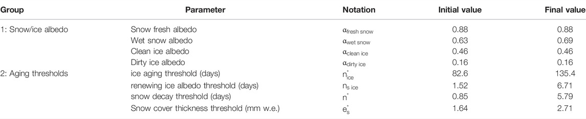
TABLE 2. Albedo parameters after calibration completed. The initial snow/ice albedos (initial value) and aging threshold values (final value) were taken from Gurgiser et al., 2013a and Maisincho (2015), respectively.

3.1.4 Temperature Lapse Rate

To represent the decrease in air temperature as a function of altitude, we determined a temperature lapse rate (TLR) of = −5.5°C (km)⁻¹ for the site. This value was obtained by linear regression between the mean values measured at each SAMA stations’ location (see Supplementary Table SA2). Therefore we ensure to capture the mean spatial variability over the glacier and avoid deviations that could cause the inclusion of values from moraine terrain which experiment large daily variations. The computed gradient matches with the value commonly employed to extrapolate air temperature in the outer tropics (Sicart et al., 2011; Gurgiser et al., 2013a) and was similar to the −5.4°C (km)⁻¹ found by Ceballos et al. (2012) for colombian glaciers in the inner tropics.

3.1.5 Roughness Parameters

The aerodynamic (z_0m) and scalar (z_0T, z_0q) roughness lengths play an essential role in the evaluation of turbulent heat fluxes using the bulk method (e.g., Favier et al., 2011). Turbulent heat fluxes are very sensitive to the choice of these parameters (Wagnon et al., 1999; Hock and Holmgren, 2005), and surface roughness lengths are often obtained by calibration using field measurements (e.g. Wagnon et al., 1999, 2003; Favier et al., 2004a). It is often easier to fix the values of equal roughness (z_0m = z_0T = z_0q) as considered in several studies in the tropics. In this case, roughness lengths lose their physical meaning. For the AG12 site, we used a value of z_0m = z_0T = z_0q = 2.9 mm for the ice, which corresponds to the value calibrated in the ablation zone of AG15 by Favier et al. (2004a). A value of z_0m = 4 mm was used for snow (Wagnon et al., 1999). In the case of a precipitation event, the roughness length of fresh snow is reduced to 0.29 mm during the current time-step (Gurgiser et al., 2013a).

3.2 Distributed SEB Model

Initially, the model was applied locally at the SAMA-1 altitude level, where the model parameters were calibrated. This step was particularly important for the albedo model. Then, the model was distributed over 20 different 50-m altitude bands. For this purpose, the incident short-wave radiation (SWi) was corrected according to the mean slope (β_i) and the mean aspect (Az_i) of the corresponding band. These values were computed from the DEM pixels located between z_i − 25 and z_i + 25. The representative area (A_i) on which the energy balance was calculated corresponds to the number of pixels in the band multiplied by the individual area of one pixel (100 m²) and by the cosine of the slope.

Calculations were performed with a 30-min time step for each band (i), following the order of operations described below: 1) we first calculate the incident short-wave radiation SWi(z_i) as a function of surface slope (β_i) and azimuth (Az_i), 2) we extrapolate the air temperature for each band using temperature lapse rate, the air temperature (Tz_ref) measured at the SAMA-1 station located at the reference altitude z_ref = 4,753 m a.s.l., and the altitude (z_i) of the considered band, 3) using Stephan Boltzmann equation, we correct the LWi values as a function of altitude considering that the variations depend on air temperature only T(z_i) 4) we evaluate the precipitation as a function of altitude z_i, 5) we discriminate the precipitation phase as a function of T(z_i), 6) we model the snow accumulation and the albedo, 7) we evaluate the value of the short-wave radiation reflected by the surface SWr (z_i), 8) we calculate the turbulent fluxes for the corresponding T(z_i), surface roughness length and surface temperature T_s(z_i) value from the preceding calculation time step 9) we compute the available surface energy E_surface, the available energy for melting G₀ and apply the thermal diffusion to obtain the melting. Thermal diffusion was computed according to an explicit scheme to a depth of 18.2 m, with a 2 cm grid resolution and a 20 s time step. After computing melting, mass balance components (e.g., solid and liquid precipitation, melting, and sublimation) were aggregated to get hourly values corresponding to the current time-step of the linear reservoir model.

3.3 Linear Reservoir Model

The transfer of meltwater and rainfall through the glacier to the outlet of the watershed is modeled using the Baker et al. (1982) model. This reservoir-type model is used to calculate the transfer from the various zones of the watershed. In our case, the watershed has been divided into four zones: three zones correspond to the glacier, which has been divided according to altitude, and a fourth zone corresponds to moraine terrain outside the glacier. Each zone is represented by a linear reservoir (Eq. 7) such that the flow rate [Q(t)] depends on a characteristic storage parameter (k) and the inflow rate [R(t)]. R(t) corresponds to the sum of melting (evaluated from the distributed SEB) and liquid precipitation. Consequently, the net discharge at the outlet results from the sum of the individual inflows.

In our approach, the “ice reservoir” refers to the lower part of the glacier, corresponding to the ablation zone. Water discharges from the central part, around the equilibrium zone, are modeled using the reservoir called “firn reservoir” hereafter; and in the upper part, where accumulation occurs, we refer to the reservoir as the “snow reservoir”. Figure 1 shows the watershed of Glacier 12 and the distribution of the different reservoirs. The boundary between the ice and firn reservoirs has been set at 5,100 m a.s.l., close to the equilibrium line altitude (Basantes-Serrano, 2015). The boundary between the firn and snow reservoirs was set at 5,300 m a.s.l., due to the change in the observed mean snow density as a function of altitude in this area (Cáceres et al., 2010).

Moreover, a reservoir corresponding to water contribution from the moraine was included in our modeling to account for the area between the glacier snout and the hydrological station (1.5 km downstream). This reservoir is fed by a permanent underground flow of Q₀ = 0.01 m³ s⁻¹ estimated from hydrological balances and salt gauging (data not shown) and to which the contribution of rainfall is added and is proportional to precipitation (measured with the rain gauge P8) according to PSO and to the surface area of this zone (A_moraine). To represent the evaporation/sublimation of this zone, a stream coefficient f₀ = 0.8 was included. Thus, the inflow [R₀(t)] for this reservoir was represented by Eq. 8.

Heavy precipitation sometimes produces a snow cover that can persist from a few hours to a few days over the entire watershed, resulting in short-term water storage. Nevertheless, the parameters for sizing the storage in the reservoir model were considered constant because the snow stored in the lowest part of the watershed was considered negligible, but also because the model is only a conceptual representation allowing to compute the water amount delivered at the hydrological station. Studying the exact origin of the inflow is not a focus here. Thus, the storage corresponding to the snow is indirectly integrated into the calculation of the reservoir parameters when the model is calibrated (Hock, 2005).

The model parameters corresponding to the water storage were calibrated using a Monte-Carlo-type approach carried out on 10⁴ simulations for which all the parameters had randomly estimated values. This calibration of the time of responses (k) was performed over the 2012 period, and the validation was carried out over the July-December 2011 plus January-May 2013 period. The optimal values selected are those that maximize the coefficient of determination calculated between the observed and simulated discharges. Table 3 shows the final parameter values obtained. The ranges of variation of the parameters were defined according to the values applied in linear reservoir models on other glacial basins (Cuffey and Paterson, 2010). A sensitivity analysis was not performed because the simulated discharge using the linear reservoir model is not strongly dependent on the parameters associated with storage (Hock and Noetzli, 1997).

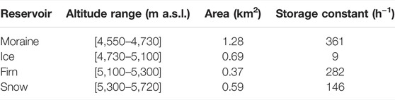
TABLE 3. Altitude range, area, and storage constants used for the linear reservoir model. In the approach the altitude for each reservoir were kept fix since most of snowfalls at site are short-lived.

4 Results

4.1 Meteorological Conditions

4.1.1 Observed Values During SP

During SP, the air temperature and specific humidity at SAMA-1 oscillated around the mean values of 1.31°C and specific humidity of 5.8 g kg⁻¹, respectively. They presented a slight maximum between February and May (1.66°C, 6.7 g kg⁻¹) related to the equinox characterized by a higher cloud cover and weaker wind conditions. In contrast, a slight drop in both variables was observed from June to September (0.75°C and 5.2 g kg⁻¹, respectively). These differences are minimal compared to the standard deviation of daily values (1.81°C and 1.2 g kg⁻¹), reflecting the lack of marked thermal seasonality in Ecuador (Kaser and Osmaston, 2002). The cloud factor (CF) showed values above 0.6 during the two periods of heavy precipitation (February-May and October-December); therefore these periods were characterized by lower values of SWi and large values of LWi (Figure 3). On the contrary, the mean wind speed was 3.8 m s⁻¹ (σ = 2.4 m s⁻¹), with June-September season marked by stronger easterly winds (mean = 6.7 m s⁻¹, σ = 3.3 m s⁻¹), thus reducing cloud cover leeward the volcano (CF = 0.2) which in turn reduced LWi and increased SWi.

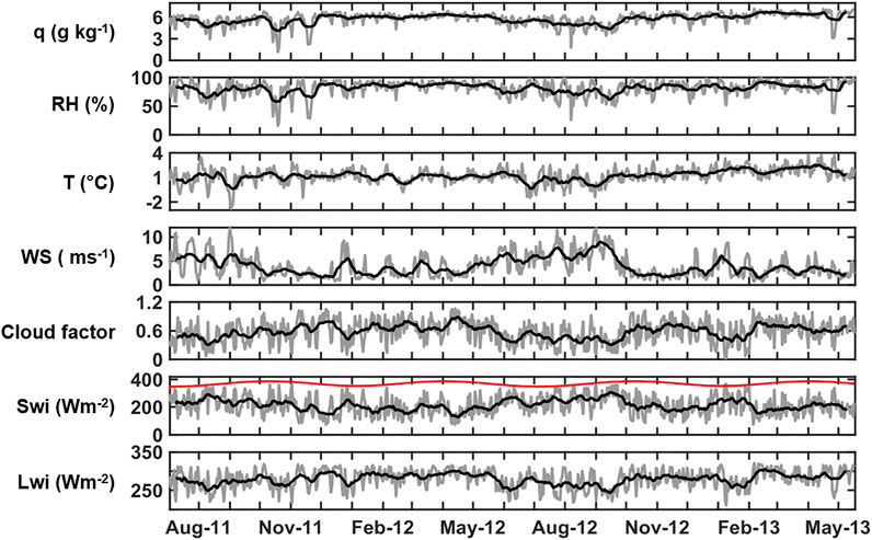
FIGURE 3. Summary of daily mean (gray line) meteorological conditions measured at AWS SAMA-1 (4,753 m a.s.l.). Thick black lines represent the 15-day running means. The red curve shows theoretical solar radiation at the top of atmosphere (STOA) reduced by 50 Wm⁻² and represents maximums theoretical radiation on clear days. The cloud factor CF (dimensionless) was calculated as the ratio between the incoming short-wave radiation and STOA according to Eq. 1.

P8 rain gauge collected 1,429 mm and dry days accounted for 28% of the SP. Periods without precipitation never exceeded 10 days. Thus, demonstrating the prevalence of rainy conditions. Using the PSO to separate liquid and solid precipitation (see Section 3.1.2), snowfall accounted for 757 mm corresponding to 53% of total precipitation. This value was higher than 681 mm computed using the 1°C threshold, justifying that a higher albedo value is modeled at the SAMA-1 level with the PSO approach than with a constant 1°C threshold (Figure 5).

These characteristics in temperature and radiation, as well as the precipitation cycle, affect the melting conditions, and in consequence influence the variations of the monthly discharge measured at “Los Crespos” station. Which presented an average discharge of 0.045 m³ s⁻¹ with a minimum between June and August (0.026 m³ s⁻¹) (Figure 2). On the other hand, two maxima in discharge were observed around 0.058 m³ s⁻¹ in January-May and September-November. These were associated with heavy precipitation during equinoxes and favorable conditions for significant melting (Favier et al., 2004a).

4.1.2 Representativeness of SP

In the study area, the average precipitation provided by CHIRPS was 1,298 mm (standard deviation, σ = 174 mm). The precipitation values from 2011, 2012, and 2013 differed from the mean by +2σ, −0.46σ, and −0.02σ, respectively; suggesting that 2011 was relatively wet while 2012 was slightly dry. Comparing the SP values with the corresponding monthly mean (Figure 4), five of 23 months presented values larger than one standard deviation suggesting precipitation excess, whereas 3 months were dry, i.e., with values lower than 1 standard deviation. Therefore, the study period was marked by irregular monthly precipitation with excess from July 2011 to April 2012, followed by a deficit from May 2012 to January 2013, and finally by an alternation between wet and dry months. Similarly, the mean annual temperature from ERA-5 was 1.59°C over the Antisana region (standard deviation σ = 0.74°C). 2011, 2012, and 2013 years were marked by differences with the interannual mean of +0.05σ, −0.21σ, and +0.15σ, respectively. Thus, 2012 was slightly cold, while 2013 was slightly warm. SP presented 10 months with the temperature above the respective monthly mean, and 9 months below. Thus, the study period experienced fluctuating temperatures with increasing temperature between July to November 2011, then a decrease between December 2011 and September 2012, and finally a further increase during the remaining months.

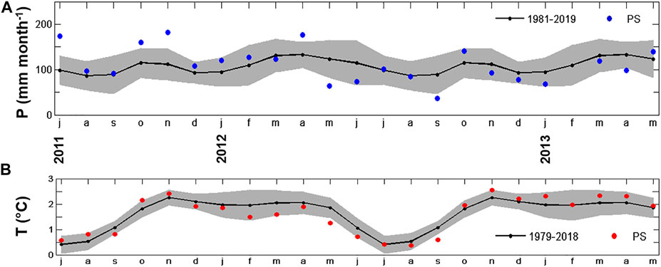
FIGURE 4. (A) Monthly CHIRPS precipitation (0.05° × 0.05°) values for the study period (blue circles) relative to mean CHIRPS precipitation for 1981–2019 period (black circles) and monthly standard deviations (gray shading) for the grid point nearest Antisana 12 Glacier (78.15°W, 0.45°S). (B) Monthly ERA5 air temperature (0.25° × 0.25°) at 600 hPa level, averaged over the Antisana massif region (0.2 to 0.8°S, 77.8 to 78.5°W) for the sudy period (red circles) relative to mean ERA air temperature for 1979–2018 period (black circles) and monthly standard deviations (gray shading).

4.2 Model Validation

4.2.1 Validation of Albedo Model

To study the role of each parameter in the albedo model a sensitivity test was carried out. The ice-snow parameters varied from 0.2 to 1.2 times the initial values taken from Maisincho (2015). These variations had an insignificant impact on the resulting albedo, except for the wet snow albedo for which high values led to a better reproduction of the daily measurements (computed between 10:00 and 16:00 local time). On the other hand, changes in the characteristic aging scales (Group 2 of Table 2) resulted in relatively random variations of the determination coefficient (Supplementary Figure S1). Then, a Monte Carlo approach based on 10⁴ simulations was performed to maximize this value computed between the daily simulated albedo and measured values. These parameters’ variation span from 0.2 to 6 times the initial values taken from Gurgiser et al., 2013a. The resulting values after calibration were summarized in Table 2.

The parameters obtained were representative of rapid snow metamorphism and faster albedo degradation in the inner tropics than in the Alps (Wagnon et al., 2009; Sicart et al., 2011). The value of the characteristic snow cover thickness at which the underlying ice surface is visible ($e_s^{\ast }$) is lower at Antisana than in the outer tropics. This point reflects the frequent presence of thin layers of fresh, wet snow due to light snowfalls, which, however, have a significant impact on albedo. Moreover, the addition of a progressive ice-albedo degradation in Eq. 5 allows taking into account a progressive accumulation of dust particles on the ice surface. This improvement is particularly significant during sporadic precipitation and for dry periods marked by a progressive decrease of the albedo until reaching the dirty ice-albedo value (Figure 5). Therefore, calibration allowed us to improve the simulations increasing the determination coefficient between measured and modeled daily albedo data, from r² = 0.13 (r = 0.36, n = 366, p = 0.17) obtained with the initial values to r² = 0.72 (r = 0.85, n = 366, p < 0.05) after calibration. The improvement was also significant for 30-min values with r² = 0.65 (r = 0.81, n = 5,124, p < 0.01).

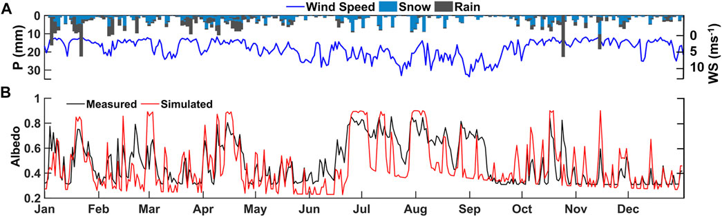
FIGURE 5. (A) Daily snow and rain values accumulated from 30-min precipitation at P8. Snowfall fraction was discriminated according to PSO scheme depending on temperature ranges (See Section 3.1.2). Daily wind speed values (blue line) measured in SAMA-1 were included for comparison purposes. (B) Comparison between daily albedo measured at SAMA-1 station (black line) and simulated after setting parameters (red line). Daily values were computed in the daytime between 10:00 and 16:00 h local time.

Since albedo controls variations of the net short-wave radiation (Favier et al., 2004a), these changes significantly improved the representation of this energy flux, which controls the energy available at the surface and thus the melt. Over the study period, the determination coefficient between modeled and measured daily melting values reached r² = 0.75 (r = 0.87, n = 686, p < 0.05), indicating good performance for long time series. There were small differences in simulated albedo between July and September (Figure 5), probably because windy conditions could redistribute the snowpack with increasing snow depth and albedo in patchy areas only. The latter process cannot be represented by the model (Maisincho, 2015).

4.2.2 Validation of Point-Based Melt Modeling

After tunning the albedo parameters, we applied the SEB model over three successive periods, called MP1, MP2, and MP3 (Table 1). These periods allowed us to test the evolution of the model quality in the ablation zone for different surface conditions. Figure 6 shows the simulated cumulative surface elevation changes for different sites around the SAMA-1. The separation between snow and rain was performed using the PSO scheme, but for comparison, the use of 1°C threshold was also tested. To quantify the differences between calculated and measured surface elevation, we compute the mean bias error (MBE) for the ablation stake locations. Since the MP2 period was short compared with MP1 and MP3, only graphical comparisons were carried out.

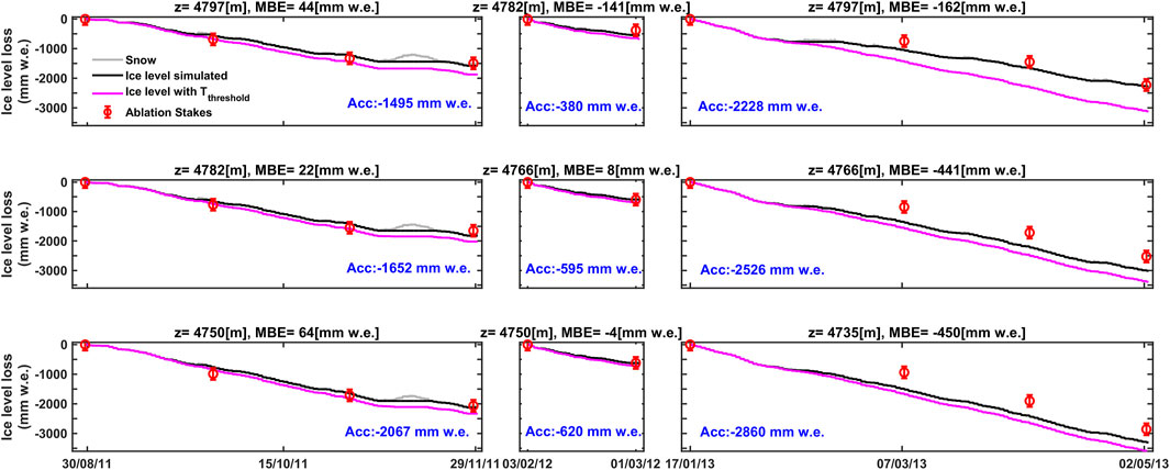
FIGURE 6. Computed and measured surface height changes for different sites (rows) during MP1, MP2, and MP3 (columns). Ice (black line) and snow (gray line) surface height were computed following the PSO scheme. Surface height measured (red circles) includes 150 mm error bars related to the measurement method. Mean bias error (MBE) between simulated and measured surface height, and cumulated height measured (text in blue) were included for each site. For comparison purposes, surface height computed with a 1°C threshold temperature (pink line) is also shown.

The MBE of the three points of MP1 was between 22 and 64 mm w.e., which corresponded to 2–4% of measured cumulative ablation, respectively. Thus, the model slightly underestimates ablation. Conversely, during the MP3, the modeled MBE was more negative than observations, with differences ranging between −450 and −162 mm w.e. suggesting that cumulative ablation was overestimated in a range of 7–17%. Using the PSO scheme, the modeled ablation got lower biases than using the 1°C threshold; especially for MP1 and MP3 both with a duration larger than 90 days. This occurred because the PSO improved the consistency between observed and modeled albedo changes due to better reproduction of solid precipitation occurrences for low-intensity events (0.5 mm w.e.) than with the 1°C threshold. This improvement was more significant for MP3 at 4,797 m a.s.l. since solid precipitation was 72 mm w.e. using the 1°C threshold, whereas it was 159 mm w.e. with PSO. This snow surplus produced a reduction in ablation of 852 mm w.e. Therefore, the additional snow was crucial to maintain the albedo above 0.3 and thus to avoid overestimating ablation.

4.2.3 Validation of the Distributed Modelling

The variations of the mass balance with elevation were simulated and compared with those of the observed geodetic mass balance (Figure 7). By examining the mass balance profiles with elevation, most of the simulated values were very close to the measurements. The distributed SEB model overestimated 15% of the ablation in the lowest zone (4,735–4,850 m a.s.l.), while it underestimated ablation by 20% between 4,850 and 5,100 m a.s.l. However, the errors in ablation modeling compensated each other, and the glacier-wide mass balance was correctly reproduced. The mass balance gradient with elevation was 22.76 kg m⁻² m⁻¹ y⁻¹ close to the 19.32 kg m⁻² m⁻¹ y⁻¹ measured, and to the 24.5 kg m⁻² m⁻¹ y⁻¹ ±5% generally applied in the inner tropics (Kaser, 2001). Between 5,100 and 5,500 m a.s.l., the model underestimated the measured accumulation by 25%, whereas it overestimated the measured accumulation by 42% in the upper part (between 5,500 and 5,720 m a.s.l.). Despite of these discrepancies in the mass balance profile modeling, the resulting glacier-wide mass balance for 2012 was −0.61 m w.e. y⁻¹, which was close to the measured value in 2012 (−0.58 m w.e. y⁻¹) and to mean rate of −0.57 ± 0.81 m w.e. y⁻¹ obtained over the period 2005–2012 (Basantes-Serrano, 2015). The distributed SEB was a priori reasonably representative of the average value observed on a 10-year scale. In section 5, we discuss why the distributed SEB could not fully represent the measured profile.

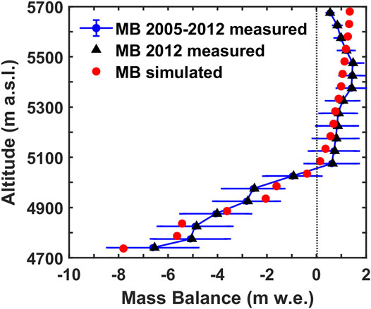
FIGURE 7. Comparison between measured and computed mass balance profiles. Blue dots represent the mean of 2005–2012 measurements, blue bars represent corresponding standard deviation for each altitude band. Black triangles represent the measurements for 2012, and red dots correspond to mass balance profile simulated. The dashed line represents equilibrium line that cross mass balance profile around 5,100 m a.s.l.

4.2.4 Streamflow Simulation

The calibrations performed on the distributed SEB and the flow transfer models allow to reproduce properly the variability of the measured discharge at a daily (r² = 0.54, p < 0.01, n = 423) and hourly (r² = 0.58, p < 0.01, n = 11,553) timescales. However, the mean simulated discharge largely overestimates the measured one. Daily mean simulated discharge was 0.187 m³ s⁻¹ (min = 0.03 m³ s⁻¹, max = 0.6 m³ s⁻¹) whereas observed discharge was 0.033 m³ s⁻¹ (min = 0.01 m³ s⁻¹, max = 0.06 m³ s⁻¹). The potential discharge was on average 5.86 times larger for the SP than the streamflow measured at the hydrological station. It is even possible that this ratio becomes 15 for some days (Figure 8). The current difference between both discharges indicates that rain and meltwaters from the glacier likely percolate into the groundwater system above the gauging station so that the streamflow at the gauging station is lower than expected. This occurrence of significant groundwater flow had already been observed in the case of the AG15 (Favier et al., 2008), showing the limits of hydrological measurements to assess the melting and mass balances of the Antisana glaciers.

FIGURE 8. (A) Comparison between simulated (blue line) and measured discharge (orange line). Only days with precipitation and discharge available are presented. (B) Scatter plot of measured vs. simulated discharge daily values. Dashed line represents the mean ratio (m = 5.86) between simulated and measured values.

Furthermore, the average contributions of each reservoir to the potential discharge were: 77% from ice zone, 14% from moraine zone, 6% from firn zone, and 3% from snow zone. These percentages confirmed that most of the runoff originated within the glacier came from the ablation zone and the nearby moraine. Therefore, the contribution of the accumulation zone was not significant.

4.3 Application of Distributed SEB Model

The model calibration step demonstrated that the coupling between the distributed SEB and water flow transfer allowed us to simulate the variations of ablation and streamflow if we assume the occurrence of significant groundwater flow circulations. Consequently, the model will be used hereafter as an analytical tool to relate weather conditions, the energy balance, and the water flows in the Los Crespos gauging station.

4.3.1 Melting, Sublimation and Discharge Peaks

In the ablation zone, as observed before on AG15 (Favier et al., 2004b), the net short-wave radiation (S = SWi − SWr) was the primary source of energy available at the surface during the study period (Figure 9), and it contributed to 53% of the absolute energy exchange. This flux was controlled by albedo variations (r² = −0.96, n = 23, p < 0.01), which in turn was related to the phase of precipitation through the snow cover thickness (r² = −0.79, n = 23, p < 0.01). Since the ice reservoir was the main provider of meltwater at the outlet, there was also a significant correlation between the potential discharge and the net short-wave radiation (r² = 0.80, n = 23, p < 0.01). The correlations between the potential discharge and other components of the SEBs were not significant (r² always lower than 0.4, p > 0.05), demonstrating that the outflow was not highly dependent on these other fluxes. However, despite a significant seasonality of the short-wave radiation at the top of the atmosphere (STOA), the presence of cloudiness and precipitation during the study period attenuated the seasonality of SWi (Figure 3), and no seasonality was found in the variation of discharge during SP.

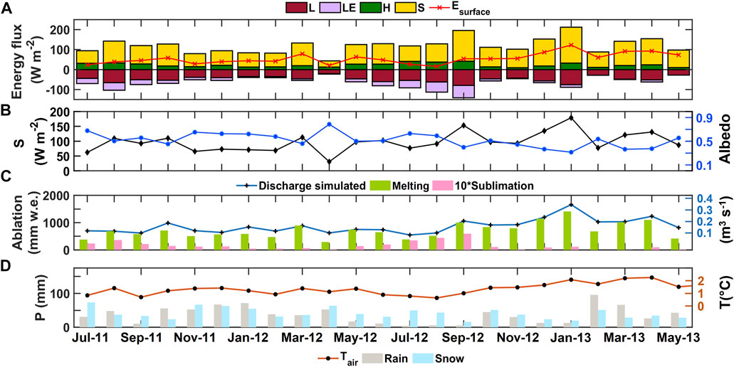
FIGURE 9. (A) Monthly values of the surface energy balance components and resulting energy available at surface (red line) for the 4,780 m a.s.l. band nearest to SAMA-1. (B) Comparison between net short-wave radiation (black line) and albedo (blue line) at 4,780 m a.s.l. (C) Monthly discharge simulated (blue line), accumulated melting (green bars) and sublimation (pink bars) at 4,780 m a.s.l. For visualization purposes, sublimation was multiplied by a 10 factor. (D) Monthly air temperature measured in SAMA-1 (brown line) and accumulated snow and rain measured in P8. Separation phase was determined through PSO scheme.

Moreover, the location of the Antisana massif in the vicinity of the Amazon basin allows the glacier to continuously receive the moisture transported by the easterlies (Junquas et al., 2022). During SP, this induced the presence of significant cloud cover throughout the year and finally reduced the seasonality in LWi (Table 3). Also, the homogeneity of air temperature (Section 2.1) allowed the glacier surface to be at the melting point most of the time (Francou et al., 2004), and LWo was regular. As consequence, the longwave radiation also presented no seasonality (Figure 9). Since the radiative fluxes (S + L) contributed 80% of mean absolute energy during SP, the E_surface and mass balance neither exhibited seasonality in accordance with their low coefficient of variability (CV = 0.5) and low standard deviation (Table 3). The lack of seasonality in SWi and LWi also implies that SWr and LWo variations drove S and L and were key in determining the available energy for melting. Considering that SWr are related to albedo and snowpack thickness, it justifies that glaciers in the inner tropics are very sensitive to air temperature through its influence on the precipitation phase (Favier et al., 2004a; Favier et al., 2004b; Francou et al., 2004).

Finally, to illustrate the influence of weather conditions on discharge variations, we related it with the energy fluxes at SAMA-1 during the months of maximum/minimum energy available for melting. During April 2012, the net short-wave radiation (S = 43 W m⁻²) was minimal (Figure 9) due to continuous cloud cover (CF = 0.95) and solid precipitation, SWi was reduced and a significant snow cover (64 mm) was present at the surface leading to an increase in the albedo up to 0.8. With very high SWr, the net short-wave radiation dropped leading to low melting amounts and discharge. Similarly in July 2012, low air temperature and significant precipitation provided fresh snow at the surface, which sustained a high albedo and low S value. In addition, seasonal high wind speed (Ws = 6.62 m s⁻¹) favored a large turbulent latent heat flux, which is an efficient energy sink. Both conditions reduced the available energy to 26 W m⁻². Thus, melting and discharge were minimum (around 380 mm w.e. and 0.09 m³ s⁻¹, respectively), and 47% lower than their respective mean values over SP. Conversely, January 2013 presented low cloud cover (CF = 0.45) and high precipitation deficit yielding high SWi and low SWr, which resulted in maximum short-wave radiation (S = 179 W m⁻²). Moreover, the air temperature was high (T = 1.85°C), favoring a positive turbulent sensible heat flux (H = 32 W m⁻²) toward the glacier surface. Then, the available energy was maximal (E_surface = 122 W m⁻²), causing a peak in melting (1,414 mm w.e.) and discharge (Q = 0.37 m s⁻¹) (Figure 9) corresponding to overflow of 99 and 119% with respect to their respective mean values.

4.3.2 Variation in Energy Fluxes According to Elevation

Figure 10 shows the dependence of energy fluxes on altitude. A reduction of the net short-wave radiation resulted from the occurrence of greater snowfall amounts at high elevations. Frequent snowfalls maintained the albedo above 0.7 (high SWr). The concave shape of the glacier also contributed to this result because the zenithal angle increases with the slope, thus reducing SWi. The net short-wave radiation decreased from 120 W m⁻² at the glacier front to 30 W m⁻² at 5,100 m a.s.l. Above this altitude, its decrease was less significant, reaching 26 W m⁻² at the summit. In addition, the drop in air temperature induced a reduction of the LWi from 281 W m⁻² at the front of the glacier to 247 W m⁻² at the summit. This decrease was partially offset by the reduction in LWo due to the drop in surface temperature (T_s). Thus, the net longwave budget passed from −33 W m⁻² at 4,735 m a.s.l. to −47 W m⁻² at 5,100 m a.s.l. This reduction continued almost linearly with the altitude until reach −67 W m⁻² at the summit.

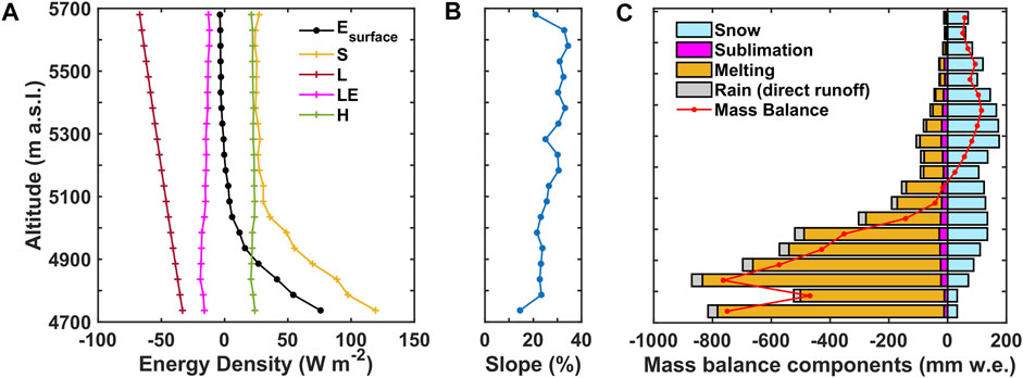
FIGURE 10. (A) Mean variation of energy fluxes with altitude during SP. (B) Variation of surface slope with altitude resulted from the DEM analysis. (C) Altitudinal profile of components of specific mass balance for SP.

Since the decrease of T_s was linked to the radiative flux decrease with altitude, the temperature gradient between air temperature above the surface and T_s remained almost constant. In consequence, the sensible turbulent heat was constant with an elevation of around 23 W m⁻². Similar behavior occurred with the specific humidity gradient. Therefore, the latent heat did not evolve significantly with elevation and remained around −15 W m⁻². The changes in turbulent fluxes between 4,900 and 5,000 m a.s.l. were related to changes in the surface roughness length due to the surface transition from ice and snow. Assuming constant wind speed profile with elevation (measured at SAMA-1) resulted in a slight variation of turbulent fluxes. However, this assumption propagates uncertainties to higher altitudes where stronger wind should drive higher turbulent fluxes values (Dadic et al., 2013).

The variation of SEB components resulted in a decrease of E_surface from the glacier snout to the ELA (5,100 m a.s.l.) such that the net short-wave radiation and the turbulent sensible heat flux prevailed in the ablation zone and provided 21 W m⁻² of energy to the surface for melt, on average. In addition, 64% of the melting occurred directly at the surface, while the remaining 36% occurred in the sub-surface layer. This may explain the observed 5–10 cm deep cryoconite holes in the field. The ablation zone received 74% of total rain and 33% of total snow; but accounted for 91% of melting amount and 46% of sublimation, respectively. Although the highest melting rate occurred at the glacier snout, the largest contribution came from the 4,850 m a.s.l. altitude band (Figure 10), in accordance with the major exposure area at the ablation zone. Since the turbulent heat fluxes and net radiation compensated each other in the accumulation zone, there was unimportant melting in this zone. Then, mass losses at high elevation were mainly by sublimation. The highest snow accumulation occurred at the summit, but the zone of maximum accumulation took place at 5,300 m a.s.l. due to the widest surface area at this altitude.

4.3.3 Relationship Between Mass Balance and Potential Streamflow

Figure 11 shows the monthly variation profiles of E_surface and surface mass balance as a function of altitude, as well as the volume of water from each reservoir. During SP, the average monthly ablation was −0.24 m w.e. between 4,735 and 5,100 m a.s.l. (−0.65 m w.e. at the glacier snout), corresponding to a mean discharged volume of 4.38 × 10⁵ m³ with 77% coming from the ice reservoir. Months with the lowest precipitation (less than 40 mm) like September 2012, December 2012, and January 2013 were associated with a higher mass loss (−0.52 m w.e.) generating larger meltwater volumes around 7.22 × 10⁵ m³ with 86% of the contribution from ice reservoir. Indeed, September 2012 was characterized by the maximum wind speed (Ws = 6.8 m s⁻¹), and the lowest specific humidity (q = 4.8 g kg⁻¹) that maximized the turbulent fluxes (H = 42 Wm⁻², LE = −62 Wm⁻²). Sublimation (59 mm w.e.) was promoted by dry conditions, but low precipitation (21 mm) led to a low albedo leading to intense ablation.

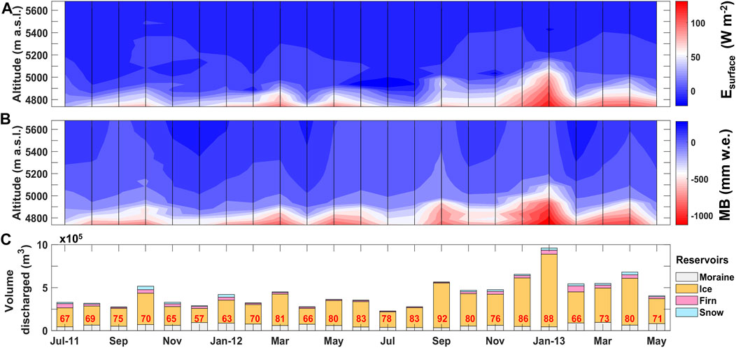
FIGURE 11. (A) Monthly profile of surface energy available at surface. (B) Monthly mass balance profile. (C) Monthly discharge cumulated at each reservoir. Numbers in red represents the ice reservoir contribution concerning total discharge.

By contrast, months with precipitation exceeding 90 mm like July, November and December 2011, and April 2012 were marked by limited mass losses (−0.16 m w.e. on average), resulting in 3.1 × 10⁵ m³ volume discharged such that ice reservoir contributed with 64% of the potential discharge. The two latter months were thus possibly marked by mass gains in the accumulation zone (0.14–0.21 m w.e.). In general, the melting above the ELA was limited because significant sublimation sank E_surface. Hence, firn and snow reservoirs contributed with the 6 and 3%, respectively, of the potential discharge. Whereas below this altitude, the ice reservoir concentrated most of the melting. In general, the contribution of ice and moraine reservoirs depended on the rain/snow ratio because months with greater snowfall occurrence than rain limited the contribution from the moraine and increased the contribution of the ice reservoir up to 80% (Figure 11).

5 Discussion

5.1 Comparison of Antisana Glacier 12 SEB With Other Tropical Glaciers

We compared the meteorological conditions and SEB values at the AG12 (Table 4) with those reported at AG15 by Favier et al. (2004a). Slight differences were found. AG12 presented lower SWi and slightly larger LWi than at AG15. Indeed, moisture transported by the wind can condense at the summit and along the upper slopes on the western side of the volcano (Basantes-Serrano et al., 2016), producing a cloud cover on the AG12. Whereas along the northern flank, this air flux preferably passes without producing clouds, and AG15 is more frequently under clear sky conditions. Also, the windy conditions and cooler temperatures in AG15 are explained by the higher location of the AWS (125 m higher than on AG12). Therefore, local features linked to the aspect and morphology of the glacier increased energy losses of AG15 via L and LE and reduce melting and ablation than on AG12.

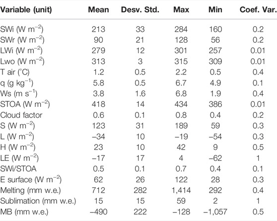
TABLE 4. Summary of Mean monthly values of meteorological and SEB variables at SAMA-1 location during SP. Des. Std. and Coef. Var. refer to standard deviation and coefficient of variation, respectively.

These differences do not alter the low seasonality of energy fluxes and became less important at the interannual scale. Hence, both glaciers share similar responses and mass balance trends (−0.46 m w.e. y⁻¹ for AG15 vs. −0.57 m w.e. y⁻¹ for AG12 for 2005–2012 records) rough to the −0.6 m w.e. y⁻¹ estimated by Rabatel et al. (2013) to the tropical glaciers. Therefore, results in AG12 can be used as a first proxy to determine the meltwater production and mass balance of Cayambe and Cotopaxi glaciers located in the Eastern Cordillera, which share similar climatic conditions. Conversely, the Chimborazo volcano is located in the Western Cordillera and holds less-humid conditions (550–750 mm/year) with a marked dry season between June-September (Ilbay-Yupa et al., 2021). Thus, Chimorazo’s glaciers present more negative mass balance and additional melting reaching 1.5 m w.e. below their ELA (5,050 m a.s.l) according to Saberi et al. (2019).

In addition, the meteorological conditions and SEB components of AG12 were compared with those reported in Artesonraju glacier (Peru) (Juen, 2006) and Zongo glacier (Sicart et al., 2011). The air temperature at all sites presented low seasonal variability characteristic of tropical glaciers. However, the vicinity of AG12 to the moisture sources explains the larger values of specific humidity, cloudiness, and LWi than all the other sites (Supplementary Table S1). The wet conditions make the turbulent latent heat flux constant and prevent nocturnal radiative cooling maintaining the surface glacier temperature close to 0°C. Thus, energy balance and melting depend mostly on short-wave radiation, except during the June-September season when strengthen Easterlies increase the sublimation and melting is reduced, similarly as observed on Artesonraju glacier. In addition, the variation of SEB components with altitude modeled in AG12 followed the same behavior of the values at Shallap glacier (Gurgiser et al., 2013a), especially the turbulent heat fluxes. This was expected since Shallap and Antisana glaciers present quite similar conditions. Conversely, Zongo Glacier is characterized by a very marked seasonality of LWi, especially during the June-September season; where very large sublimation amounts are not compensated by the solar radiation and melting is then negligible (Favier et al., 2004b).

5.2 Influence of Temperature Lapse Rate and Precipitation Correction

To analyze the effect of TLR and precipitation factors on the mass balance profile we investigate some schemes to extrapolate these variables over the glacier. The linear regression between mean temperature values at SAMA-1, 2, and 3 leads to a lapse rate of −5.5°C km⁻¹ (see Section 3.1.4.); also, we try with −5.9°C km⁻¹ corresponding to the median value of TLRs computed from 30-min sets measured simultaneously for the three SAMA stations. Concerning precipitation corrections, we tested four configurations: 1) constant precipitation with elevation without including a correction for wind-induced under-catch 2) constant precipitation with elevation including a 23% correction to account for the under-catch of hydrometeors (see Section 3.1.1) 3) same as configuration 2 but we added a precipitation gradient with the altitude of 40 mm per 100 m as proposed Basantes-Serrano et al., 2016 to match measured mass balances in the accumulation zone of AG15, and 4) same as configuration 2 but we include a linear increase of 10% every 100 m in altitude. Thus, the 837 mm cumulated annually at P8 would increase to 1,450 mm at the summit (e.g., a 73% factor) with configuration 3; whereas configuration 4 enhances an increase from 837 to 2,059 mm at the summit (e.g., a 146% factor).

All configurations were applied to assess the mass balance simulated during 2012 (Figure 12). The schemes employing constant precipitation and with/without correction for under-catch resulted in more significant mass balance losses and located the ELA 300 m above its real altitude. Thus, a vertical increase of precipitation is critical to match the mass balance with measurements. Recently, Junquas et al., 2022 has found the spatial precipitation maximum occurs at the Antisana summit with maximum values preferably on the windward side of the mountain. This reinforces the need of employing a scheme to represent the correction of precipitation with elevation. Adding 40 mm per 100 m⁻¹ gives accurate point mass balance in the ablation zone, but underestimated the accumulation between 5,100 and 5,500 m a.s.l. This was not the case with the 10% linear increase, which proposed the best fit with data measured along the entire altitudinal profile.

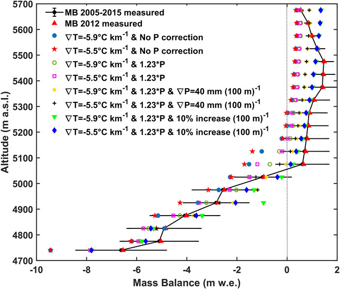
FIGURE 12. Variation of simulated mass balance 2012 profile to changes in temperature lapse rate and precipitation correction schemes. Scheme with $\nabla T=-5.5°\text{C}{\text{km}}^{-1}$ and 10% (100 m)⁻¹ linear increase of corrected precipitation by 1.23 factor used for simulating distributed SEB got the minimum RMSE.

Concerning the temperature lapse rate, we observed TLR of −5.9°C km⁻¹ leads to underestimating ablation with elevation with the largest bias observed between 4,900 and 5,050 m a.s.l. Above this elevation range, both TLR gives similar mass balance because melt becomes negligible. Therefore, TLR of −5.9°C km⁻¹ may be less representative because it was derived from a smaller dataset of air temperature measurements (N = 1,224). Conversely, the TLR of −5.5°C km⁻¹ produced fewer deviations since this value was derived with a larger dataset available (N = 54,683, 28,713, and 8,297 for SAMA-1, -2, and -3, respectively), thus allowing a better representation of glacier conditions. Overall, the best fit between simulated and observed MB (RMSE = 0.55 m w.e.) is obtained with the value of −5.5°C km⁻¹, and considering that precipitation increases linearly with elevation at a rate of 10% (100 m)⁻¹. This temperature lapse rate is close to the value −5.1°C km⁻¹ computed by Erazo (2020) for interpolations above 5,500 m a.s.l. in the Ecuadorian Andes. Moreover, this precipitation increase factor used to balance the accumulation has also been used in distributed SEB modeling in the Tropical Andes (Autin et al., 2021; Lozano Gacha and Koch, 2021). However, new accumulation measurements should be necessary to validate this precipitation rate since accumulation is particularly difficult to assess in the accumulation zone of Antisana glaciers (Basantes-Serrano et al., 2016).

In the distributed SEB model, the implementation of refreezing scheme was neglected because the glacier surface in the ablation zone stays at the melting point most of the time (Francou et al., 2004) and because most melt is concentrated under ELA. Finally, here we did not analyze the influence of the variation of wind speed and specific humidity with altitude because the measurements available at SAMAs stations did not overlap during SP. Also, since these variables are prone to local variations, due to the influence of boundary layer effects and topographical disturbances (Zardi and Whiteman, 2013), the resulting relationships with altitude are more complex than linear interpolations used in temperature. Thus, the lack of additional measurements along the altitudinal profile did not allow us to propose realistic gradients on Antisana volcano. The available measurements show the mean wind speed on SAMA-3 (5,065 m a.s.l.) was 6.2 m s⁻¹ (Supplementary Table SA4) twice as high as at SAMA-1. Whereas the mean decrease in specific humidity was about 4% between the same stations (Supplementary Table SA3). Considering that higher wind speed and lower specific humidity increase turbulent fluxes (Dadic et al., 2013), the use of invariant values of Ws and q along the glacier profile could lead to underestimating turbulent fluxes and sublimation in the upper part.

5.3 Groundwater Flow

Despite simulated discharge values being significantly higher than measured values (Table 5), we observed a significant correlation between the two variables. This reflects the close relationship between albedo and discharge fluctuations. A large part of meltwater from the ablation zone (0.69 km²) likely flows through moulins and crevasses and percolates into subglacial channels that connect with a groundwater flow network. This phenomenon has already been described for ice-covered watersheds (Hayashi, 2020; Somers and McKenzie, 2020; Miller et al., 2021), and is particularly significant at the AG15 as shown by Favier et al. (2008).

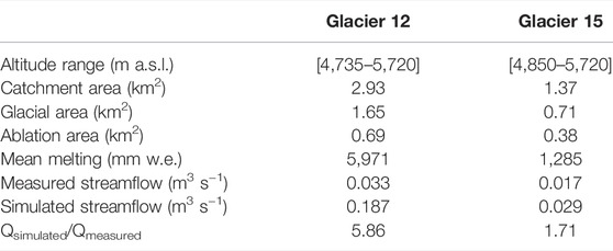
TABLE 5. Comparisons of hydrological features between Antisana Glacier 12 for 2012 year using distributed SEB plus linear reservoirs and Antisana Glacier 15 for 1995–2005 period using semi empirical approach taken from Favier et al. (2008).

The high correlation values between modeled and measured discharges suggest the flow measured at the proglacial gauging station probably originates from a minor proportion of the glacier, which is likely at lower elevations. Indeed, if percolation in the groundwater flow system were significant beneath the entire glacier, it would absorb all meltwater during periods of low melt. Then, the discharge would reflect no diurnal variation during periods of low melt. This is not the case in Figure 8A, moreover, meltwater probably flows directly to the gauging station, without entering in a porous medium, as suggested by the short delay between melt onset and peak flow at the gauging station. Perhaps, the circulation of water in a porous medium, within the moraine, would filter the flow response and attenuate flow fluctuations (Wagnon et al., 1998; Flowers, 2008). These observations were already suggested by tracer experiments performed by Favier et al. (2008), but the present modeling approach offers a better understanding of water origins. Retrieving the exact origin of meltwater is, however, a challenging task relying on complex geophysical surveys and water chemical tracing experiments (Harrington et al., 2018; Vittecoq et al., 2019). This would be relevant to accurately characterize the hydrological drainage system on the Antisana.

Direct comparisons had shown the glacier streamflow from Los Crespos gauging station contributes 22% on average (ranging between 10 and 30% according to the season) to the watershed outlet at downstream (Villacís, 2008). However, hydrograph separation based on electroconductivity, and isotopic tracers showed glacier contribution could rise to 40% of streamflow at outlet during precipitation events (Minaya et al., 2021). The calculation of hydrological balances at the scale of the massif would be necessary to find out if the underground flows are effective at lower altitudes. Studies conducted on the Quilcay river, a 3,925 m long study reach between 3,910 and 4,040 m.a.s.l. (Cordillera Blanca, Peru), have shown 49% of the streamflow is exchanged with the subsurface, with the net groundwater contribution to the discharge at the outlet about 29% (Somers et al., 2016). Thus, it is essential to develop hydrogeological studies to better understand the hydrological processes in the Antisana massif.

6 Conclusion

The impact of climatic variations on the extent of glaciers in the inner tropics has been of growing interest in recent years because of their quick response to temperature and precipitation variations. In this work, we coupled the distributed surface energy balance with a linear reservoir to quantify the potential discharge produced by melting over the entire glacier including moraine zone. In addition, the variation of discharge was related to meteorological conditions by energy fluxes. The use of precipitation partitioning based on temperature ranges instead of temperature threshold improved the mass balance simulations. Moreover, the sensitivity analysis demonstrated the need of including an increase in precipitation of 10% per 100 m increase in altitude to reproduce correctly the mass balance profile. Therefore, sequential calibrations allowed us to control the SEB model performance and best reproduce the integrated melting at the glacier scale.

It was verified that the net short-wave radiation was the main energy input for melting in the ablation zone, where 91% of the meltwater and 86% of discharge are produced. This explains the significant correlation between this flux and the simulated discharge. The lack of significant seasonality in cloud cover and in the incident short-wave radiation implies that reflected short-wave radiation rules the melting variations. This explains why albedo variations via the snow thickness regulate ablation in the inner tropics. During the July-September season, the strength of Easterlies dissipates cloud cover, and the wind speed and low specific humidity become more relevant to control melt variations due to a high turbulent latent heat flux.

The existence of groundwater flow occurring directly below the glaciers prevents us from directly comparing the amount of simulated meltwater with the measured discharge values at the hydrological gauging station. However, the high correlation between them at daily and hourly time steps ensures the model could reproduce satisfactorily the main processes influencing discharge variations. Moreover, we propose that the meltwater flowing at the gauging station comes primarily from a limited area in the lowest parts of the glacier. Hydrogeological studies are needed to complete the glacial modeling and define the area of the glacier contributing to downstream flow.

Finally, these results will allow a better understanding of the differences in the behavior between glaciers located along the Andes of Ecuador. An analysis over a longer period would now be interesting to analyze the interannual variations of energy fluxes, and their links with climate variability, in particular with ENSO; which is the main climatic driver in the zone.

Data Availability Statement

The raw data supporting the conclusions of this article will be made available by the authors, without undue reservation.

Author Contributions

LG conducted the literature review, results and analysis. LG and J-CR-H wrote the draft of the manuscript. VF and LM performed the model development. MV and LC supervised the work and mentored LG. LM conducted field work and data acquisition. J-CR-H, VF, and TC provided technical contributions and contributed to the manuscript edition. All authors contributed to the article and approved the submitted version.

Funding

Financial support received from Escuela Politécnica Nacional (EPN) by the projects EPN-PIMI-14-06 and EPN-PIJ-18-05 for the development of this research. Also, financial support for field survey received by French Research Institute for Development (IRD) through the International Laboratory LMI GREAT-ICE.

Conflict of Interest

The authors declare that the research was conducted in the absence of any commercial or financial relationships that could be construed as a potential conflict of interest.

Publisher’s Note

All claims expressed in this article are solely those of the authors and do not necessarily represent those of their affiliated organizations, or those of the publisher, the editors and the reviewers. Any product that may be evaluated in this article, or claim that may be made by its manufacturer, is not guaranteed or endorsed by the publisher.

Acknowledgments

The authors thank the Escuela Politécnica Nacional (EPN) and Instituto Nacional de Meteorología e Hidrología (INAMHI) through the project SENACYT-EPN PIC-08-506 for the support provided to install and operate the AWS SAMA-1. To the INAMHI research program Glaciares Del Ecuador and the MsC. Bolívar Cáceres for the glaciological information provided. To the GLACIOCLIM Observation Service for the information on the E-ORE station used, and to Ruben Basantes for the glaciological and geographical information provided. J-CR-H thanks to Secretaría Nacional de Educación Superior, Ciencia, Tecnología e Innovación, SENESCYT for financial support through a PhD scholarship. The authors acknowledge Juan Carvajal for the field data acquisition.

Supplementary Material

The Supplementary Material for this article can be found online at: https://www.frontiersin.org/articles/10.3389/feart.2022.732635/full#supplementary-material

References

Anslow, F. S., Hostetler, S., Bidlake, W. R., and Clark, P. U. (2008). Distributed Energy Balance Modeling of South Cascade Glacier, Washington and Assessment of Model Uncertainty. J. Geophys. Res. 113 (2), 1–18. doi:10.1029/2007JF000850
Autin, P., Sicart, J. E., Rabatel, A., and Soruco, A. (2021). Climate Controls on the Interseasonal and Interannual Variability of the Surface Mass Balance of a Tropical Glacier (Zongo Glacier, Bolivia, 16°S): New Insights from the Application of a Distributed Energy Balance Model over 9 Years. Earth Space Sci. Open Archive. [Manuscript submitted for publication]. doi:10.1002/ESSOAR.10507310.1
Azam, M. F., Ramanathan, A., Wagnon, P., Vincent, C., Linda, A., Berthier, E., et al. (2016). Meteorological Conditions, Seasonal and Annual Mass Balances of Chhota Shigri Glacier, Western Himalaya, India. Ann. Glaciol. 57 (71), 328–338. doi:10.3189/2016AoG71A570
Baker, D., Escher-Vetter, H., Moser, H., Oerter, H., and Reinwarth, O. (19821982). A Glacier Discharge Model Based on Results from Field Studies of Energy Balance, Water Storage and Flow (Vernagtferner, Oetztal Alps, Austria). Hydrological Aspects of Alpine and High-Mountain Areas. Proc. Exeter Symp. 138, 103–112.
Basantes-Serrano, R. (2015). Contribution à l’étude de l’évolution des glaciers et du changement climatique dans les Andes équatoriennes depuis les années 1950 [Université Grenoble Alpes, PhD dissertation, 207. Available at: http://theses.fr/2015GREAU009.
Basantes-Serrano, R., Rabatel, A., Francou, B., Vincent, C., Maisincho, L., Cáceres, B., et al. (2016). Slight Mass Loss Revealed by Reanalyzing Glacier Mass-Balance Observations on Glaciar Antisana 15α (Inner Tropics) during the 1995-2012 Period. J. Glaciol. 62 (231), 124–136. doi:10.1017/jog.2016.17
Bayas-Erazo, M. (2020). “Understanding Ecuador's Growth Prospects in the Aftermath of the Citizens' Revolution,” in Representing Past and Future Hydro-Climatic Variability over Multi-Decadal Periods in Poorly-Gauged Regions: The Case of Ecuador [Université Paul Sabatier-Toulouse III, PhD Dissertation, 213–230. https://tel.archives-ouvertes.fr/tel-03124408. doi:10.1007/978-3-030-27625-6_9
Berberan-Santos, M. N., Bodunov, E. N., and Pogliani, L. (1997). On the Barometric Formula. Am. J. Phys. 65 (5), 404–412. doi:10.1119/1.18555
Bintanja, R., Jonsson, S., and Knap, W. H. (1997). The Annual Cycle of the Surface Energy Balance of Antartic Blue Ice. J. Geophys. Res. 102 (96), 1867–1881. doi:10.1029/96jd01801
Buytaert, W., Moulds, S., Acosta, L., De Bièvre, B., Olmos, C., Villacis, M., et al. (2017). Glacial Melt Content of Water Use in the Tropical Andes. Environ. Res. Lett. 12 (11), 114014. doi:10.1088/1748-9326/aa926c
Cáceres, B., Maisincho, L., Manciati, C., Loyo, C., Cuenca, E., Arias, M., et al. (2010). Glaciares del Ecuador, Antisana 15. INAMHI. Informe del año 2009. Informe técnico.
Cáceres, B., Francou, B., Favier, V., Bontron, G., Maisncho, L., Tachker, P., et al. (2006). El Glaciar 15 del Antisana. Diez años de investigaciones glaciológicasMemorias de La Primera Conferencia Internacional de Cambio Climático: Impacto En Los Sistemas de Alta Montaña.
Campozano, L., Célleri, R., Trachte, K., Bendix, J., and Samaniego, E. (2016). Rainfall and Cloud Dynamics in the Andes: A Southern Ecuador Case Study. Adv. Meteorology 2016, 1–15. doi:10.1155/2016/3192765
Campozano, L., Robaina, L., Gualco, L. F., Maisincho, L., Villacís, M., Condom, T., et al. (2021). Parsimonious Models of Precipitation Phase Derived from Random Forest Knowledge: Intercomparing Logistic Models, Neural Networks, and Random Forest Models. Water 13 (21), 3022. doi:10.3390/w13213022
Ceballos, J., Rodríguez, C., and Real, E. (2012). Glaciares de Colombia: más que montañas con hielo. Bogotá: IDEAM.
Chevallier, P., Pouyaud, B., Suarez, W., and Condom, T. (2011). Climate Change Threats to Environment in the Tropical Andes: Glaciers and Water Resources. Reg. Environ. Change 11 (Suppl. 1), 179–187. doi:10.1007/s10113-010-0177-6
Dadic, R., Corripio, J. G., and Burlando, P. (2008). Mass-balance Estimates for Haut Glacier d'Arolla, Switzerland, from 2000 to 2006 Using DEMs and Distributed Mass-Balance Modeling. Ann. Glaciol. 49, 22–26. doi:10.3189/172756408787814816
Dadic, R., Mott, R., Lehning, M., Carenzo, M., Anderson, B., and Mackintosh, A. (2013). Sensitivity of Turbulent Fluxes to Wind Speed over Snow Surfaces in Different Climatic Settings. Adv. Water Resour. 55, 178–189. doi:10.1016/j.advwatres.2012.06.010
Denby, B., and Greuell, W. (2000). The Use of Bulk and Profile Methods for Determining Surface Heat Fluxes in the Presence of Glacier Winds. J. Glaciol. 46 (154), 445–452. doi:10.3189/172756500781833124
Douville, H., Royer, J.-F., and Mahfouf, J.-F. (1995). A New Snow Parameterization for the Météo-France Climate Model. Clim. Dyn. 12, 21–35. doi:10.1007/BF00208760
Espinoza, J. C., Garreaud, R., Poveda, G., Arias, P. A., Molina-Carpio, J., Masiokas, M., et al. (2020). Hydroclimate of the Andes Part I: Main Climatic Features. Front. Earth Sci., 8. Frontiers Media S.A, 64. doi:10.3389/feart.2020.00064
Espinoza Villar, J. C., Ronchail, J., Guyot, J. L., Cochonneau, G., Naziano, F., Lavado, W., et al. (2009). Spatio-temporal Rainfall Variability in the Amazon basin Countries (Brazil, Peru, Bolivia, Colombia, and Ecuador). Int. J. Climatol. 29 (11), 1574–1594. doi:10.1002/joc.1791
Favier, V., Agosta, C., Genthon, C., Arnaud, L., Trouvillez, A., and Gallée, H. (2011). Modeling the Mass and Surface Heat Budgets in a Coastal Blue Ice Area of Adelie Land, Antarctica. J. Geophys. Res. 116 (3), 1–14. doi:10.1029/2010JF001939
Favier, V., Coudrain, A., Cadier, E., Francou, B., Ayabaca, E., Maisincho, L., et al. (2008). Evidence of groundwater flow on Antizana ice-covered volcano, Ecuador /Mise en évidence d'écoulements souterrains sur le volcan englacé Antizana, Equateur. Hydrological Sci. J. 53 (1), 278–291. doi:10.1623/hysj.53.1.278
Favier, V. (2004c). Etude du bilan d’énergie de surface et de la production des écoulements de fonte d’un glacier des Andes d’Equateur : Relation glacier - climat en zone tropicale. 262. [Université Montpellier 2, PhD dissertation. Available at: http://theses.fr/2004MON20200
Favier, V., Verfaillie, D., Berthier, E., Menegoz, M., Jomelli, V., Kay, J. E., et al. (2016). Atmospheric Drying as the Main Driver of Dramatic Glacier Wastage in the Southern Indian Ocean. Sci. Rep. 6 (1), 1–12. doi:10.1038/srep32396
Favier, V., Wagnon, P., Chazarin, J. P., Maisincho, L., and Coudrain, A. (2004b). One-year Measurements of Surface Heat Budget on the Ablation Zone of Antizana Glacier 15, Ecuadorian Andes. J. Geophys. Res. 109 (18), 1–15. doi:10.1029/2003JD004359
Favier, V., Wagnon, P., and Ribstein, P. (2004a). Glaciers of the Outer and Inner Tropics: A Different Behaviour but a Common Response to Climatic Forcing. Geophys. Res. Lett. 31 (16), 1–5. doi:10.1029/2004GL020654
Flowers, G. E. (2008). Subglacial Modulation of the Hydrograph from Glacierized Basins. Hydrol. Process. 22 (19), 3903–3918. doi:10.1002/HYP.7095
Francou, B., Rabatel, A., Soruco, A., Sicart, J. E. E., Silvestre, E., Ginot, P., et al. (2013). Glaciares de los Andes Tropicales: Víctimas del Cambio Climático. doi:10.13140/RG.2.1.1255.4082
Francou, B., Ramirez, E., Cáceres, B., and Mendoza, J. (2000). Glacier Evolution in the Tropical Andes during the Last Decades of the 20thCentury: Chacaltaya, Bolivia, and Antizana, Ecuador. AMBIO: A J. Hum. Environ. 29 (7), 416–422. doi:10.1579/0044-7447-29.7.416
Francou, B., Vuille, M., Favier, V., and Cáceres, B. (2004). New Evidence for an ENSO Impact on Low-Latitude Glaciers: Antizana 15, Andes of Ecuador, 0°28′S. J. Geophys. Res. 109 (18), 1–17. doi:10.1029/2003JD004484
Funk, C., Peterson, P., Landsfeld, M., Pedreros, D., Verdin, J., Shukla, S., et al. (2015). The Climate Hazards Infrared Precipitation with Stations-A New Environmental Record for Monitoring Extremes. Sci. Data 2 (1), 1–21. doi:10.1038/sdata.2015.66
Gerbaux, M., Genthon, C., Etchevers, P., Vincent, C., and Dedieu, J. P. (2005). Surface Mass Balance of Glaciers in the French Alps: Distributed Modeling and Sensitivity to Climate Change. J. Glaciol. 51 (175), 561–572. doi:10.3189/172756505781829133
Gurgiser, W., Marzeion, B., Nicholson, L., Ortner, M., and Kaser, G. (2013a). Modeling Energy and Mass Balance of Shallap Glacier, Peru. The Cryosphere 7 (6), 1787–1802. doi:10.5194/tc-7-1787-2013
Harrington, J. S., Mozil, A., Hayashi, M., and Bentley, L. R. (2018). Groundwater Flow and Storage Processes in an Inactive Rock Glacier. Hydrological Process. 32 (20), 3070–3088. doi:10.1002/HYP.13248
Hayashi, M. (2020). Alpine Hydrogeology: The Critical Role of Groundwater in Sourcing the Headwaters of the World. Groundwater 58 (4), 498–510. doi:10.1111/GWAT.12965
Hersbach, H., Bell, B., Berrisford, P., Hirahara, S., Horányi, A., Muñoz‐Sabater, J., et al. (2020). The ERA5 Global Reanalysis. Q.J.R. Meteorol. Soc. 146 (730), 1999–2049. doi:10.1002/qj.3803
Hock, R. (2005). Glacier Melt: A Review of Processes and Their Modelling. Prog. Phys. Geogr. Earth Environ. 29 (3), 362–391. doi:10.1191/0309133305pp453ra
Hock, R., and Holmgren, B. (2005). A Distributed Surface Energy-Balance Model for Complex Topography and its Application to Storglaciären, Sweden. J. Glaciol. 51 (172), 25–36. doi:10.3189/172756505781829566
Hock, R., and Noetzli, C. (1997). Areal Melt and Discharge Modelling of Storglaciären, Sweden. A. Glaciology. 24, 211–216. doi:10.3189/s026030550001219210.1017/s0260305500012192
Ilbay-Yupa, M., Lavado-Casimiro, W., Rau, P., Zubieta, R., and Castillón, F. (2021). Updating Regionalization of Precipitation in Ecuador. Theor. Appl. Climatol 143 (3–4), 1513–1528. doi:10.1007/s00704-020-03476-x
Johnson, E., and Rupper, S. (2020). An Examination of Physical Processes that Trigger the Albedo-Feedback on Glacier Surfaces and Implications for Regional Glacier Mass Balance across High Mountain Asia. Front. Earth Sci. 8, 129. doi:10.3389/feart.2020.00129
Jomelli, V., Favier, V., Rabatel, A., Brunstein, D., Hoffmann, G., and Francou, B. (2009). Fluctuations of Glaciers in the Tropical Andes over the Last Millennium and Palaeoclimatic Implications: A Review. Palaeogeogr. Palaeoclimatol. Palaeoecol. 281 (3–4), 269–282. doi:10.1016/j.palaeo.2008.10.033
Juen, I. (2006). Glacier Mass Balance and Runoff in the Cordillera Blanca, Perú. Austria: [University of InnsbruckPhD dissertation, 195.
Junquas, C., Heredia, M. B., Condom, T., Ruiz-Hernández, J. C., Campozano, L., Dudhia, J., et al. (2022). Regional Climate Modeling of the Diurnal Cycle of Precipitation and Associated Atmospheric Circulation Patterns over an Andean Glacier Region (Antisana, Ecuador). Clim. Dyn. 2021, 1–30. doi:10.1007/S00382-021-06079-Y
Kaser, G. (2001). Glacier-climate Interaction at Low Latitudes. J. Glaciol. 47 (157), 195–204. doi:10.3189/172756501781832296
Kaser, G., and Osmaston, H. (2002). Tropical Glaciers. Cambridge, United Kingdom: The Press Syndicate.
L'hôte, Y., Chevallier, P., Coudrain, A., Lejeune, Y., and Etchevers, P. (2005). Relationship between precipitation phase and air temperature: comparison between the Bolivian Andes and the Swiss Alps /Relation entre phase de précipitation et température de l'air: comparaison entre les Andes Boliviennes et les Alpes Suisses. Hydrological Sci. J. 50 (6). doi:10.1623/hysj.2005.50.6.989
Laraque, A., Ronchail, J., Cochonneau, G., Pombosa, R., and Guyot, J. L. (2007). Heterogeneous Distribution of Rainfall and Discharge Regimes in the Ecuadorian Amazon basin. J. Hydrometeorology 8 (6), 1364–1381. doi:10.1175/2007JHM784.1
Lozano Gacha, M. F., and Koch, M. (2021). Distributed Energy Balance Flux Modelling of Mass Balances in the Artesonraju Glacier and Discharge in the Basin of Artesoncocha, Cordillera Blanca, Peru. ClimateMDPI AG 9 (9), 143. doi:10.3390/cli9090143
Maisincho, L. (2015). Analyse de la fonte glaciaire et nivale dans les Andes tropicales à partir d’un bilan d’énergie: Glacier de l’Antisana, Equateur (0°28’S). [Université Grenoble Alpes, PhD dissertation. 213 pp]. Available at: http://theses.fr/2015GREAU027.
Masiokas, M. H., Rabatel, A., Rivera, A., Ruiz, L., Pitte, P., Ceballos, J. L., et al. (2020)., 8. Frontiers Media S.A, 99. doi:10.3389/feart.2020.00099A Review of the Current State and Recent Changes of the Andean CryosphereFront. Earth Sci.
Miller, J. B., Frisbee, M. D., Hamilton, T. L., and Murugapiran, S. K. (2021). Recharge from Glacial Meltwater Is Critical for alpine Springs and Their Microbiomes. Environ. Res. Lett. 16 (6), 064012. doi:10.1088/1748-9326/ABF06B
Minaya, V., Camacho Suarez, V., Wenninger, J., and Mynett, A. (2021). Runoff Generation from a Combined Glacier and Páramo Catchment within the Antisana Reserve in Ecuador. J. Ecohydraulics, 1–16. doi:10.1080/24705357.2021.2005472
Naz, B. S., Frans, C. D., Clarke, G. K. C., Burns, P., and Lettenmaier, D. P. (2014). Modeling the Effect of Glacier Recession on Streamflow Response Using a Coupled Glacio-Hydrological Model. Hydrol. Earth Syst. Sci. 18 (2), 787–802. doi:10.5194/hess-18-787-2014
Padrón, R. S., Wilcox, B. P., Crespo, P., and Célleri, R. (2015). Rainfall in the Andean Páramo: New Insights from High-Resolution Monitoring in Southern Ecuador. J. Hydrometeorology 16 (3), 985–996. doi:10.1175/JHM-D-14-0135.1
Rabatel, A., Francou, B., Soruco, A., Gomez, J., Cáceres, B., Ceballos, J. L., et al. (2013). Current State of Glaciers in the Tropical Andes: A Multi-century Perspective on Glacier Evolution and Climate Change. The Cryosphere 7 (1), 81–102. doi:10.5194/tc-7-81-2013
Ramírez, E., Francou, B., Ribstein, P., Descloitres, M., Guérin, R., Mendoza, J., et al. (2001). Small Glaciers Disappearing in the Tropical Andes: a Case-Study in Bolivia: Glaciar Chacaltaya (16o S). J. Glaciol. 47 (157), 187–194. doi:10.3189/172756501781832214
Ren, Z., Su, F., Xu, B., Xie, Y., and Kan, B. (2018). A Coupled Glacier‐Hydrology Model and its Application in Eastern Pamir. J. Geophys. Res. Atmos. 123 (2413), 613–692. 713. doi:10.1029/2018JD028572
Ruiz-Hernández, J.-C., Condom, T., Ribstein, P., Le Moine, N., Espinoza, J.-C., Junquas, C., et al. (2021). Spatial Variability of Diurnal to Seasonal Cycles of Precipitation from a High-Altitude Equatorial Andean valley to the Amazon Basin. J. Hydrol. Reg. Stud. 38, 100924. doi:10.1016/J.EJRH.2021.100924
Saberi, L., McLaughlin, R. T., Ng, G.-H. C., La Frenierre, J., Wickert, A. D., Baraer, M., et al. (2019). Multi-scale Temporal Variability in Meltwater Contributions in a Tropical Glacierized Watershed. Hydrol. Earth Syst. Sci. 23 (1), 405–425. doi:10.5194/hess-23-405-2019
Sagredo, E. A., Rupper, S., and Lowell, T. V. (2014). Sensitivities of the Equilibrium Line Altitude to Temperature and Precipitation Changes along the Andes. Quat. Res. 81 (2), 355–366. doi:10.1016/j.yqres.2014.01.008
Segura, H., Junquas, C., Espinoza, J. C., Vuille, M., Jauregui, Y. R., Rabatel, A., et al. (2019). New Insights into the Rainfall Variability in the Tropical Andes on Seasonal and Interannual Time Scales. Clim. Dyn. 53 (1–2), 405–426. doi:10.1007/s00382-018-4590-8
Sicart, J. E. (2002). Contribution à l’étude des flux d’énergie, du bilan de masse et du débit de fonte d’ un glacier tropical: le Zongo, Bolivie [Université Paris 6, PhD dissertation. 347. Available at: http://www.theses.fr/2002PA066505.
Sicart, J. E., Hock, R., Ribstein, P., Litt, M., and Ramirez, E. (2011). Analysis of Seasonal Variations in Mass Balance and Meltwater Discharge of the Tropical Zongo Glacier by Application of a Distributed Energy Balance Model. J. Geophys. Res. 116 (13). doi:10.1029/2010JD015105
Sklenár, P., Kuècerová, A., Macková, J., and Macek, P. (2015). Temporal Variation of Climate in the High-Elevation Páramo of Antisana, Ecuador. Supplementi Di Geografia Fisica e Dinamica Quaternaria 38 (1), 67–78. doi:10.4461/GFDQ.2015.38.07
Somers, L. D., Gordon, R. P., McKenzie, J. M., Lautz, L. K., Wigmore, O., Glose, A., et al. (2016). Quantifying Groundwater-Surface Water Interactions in a Proglacial valley, Cordillera Blanca, Peru. Hydrol. Process. 30 (17), 2915–2929. doi:10.1002/HYP.10912U.S
Somers, L. D., and McKenzie, J. M. (2020). A Review of Groundwater in High Mountain Environments. WIREs Water 7 (6), e1475. doi:10.1002/WAT2.1475
U.S. Army Corps Of Engineers (1956). Snow Hydrology: Summary Report of the Snow Investigations. Available at: https://usace.contentdm.oclc.org/digital/collection/p266001coll1/id/4172/.
Veettil, B. K., Wang, S., Florêncio de Souza, S., Bremer, U. F., and Simões, J. C. (2017). Glacier Monitoring and Glacier-Climate Interactions in the Tropical Andes: A Review. J. South Am. Earth Sci. 77, 218–246. doi:10.1016/j.jsames.2017.04.009
Verfaillie, D., Favier, V., Dumont, M., Jomelli, V., Gilbert, A., Brunstein, D., et al. (2015). Recent Glacier Decline in the Kerguelen Islands (49°S, 69°E) Derived from Modeling, Field Observations, and Satellite Data. J. Geophys. Res. Earth Surf. 120 (3), 637–654. doi:10.1002/2014JF003329
Villacís, M. (2008). Ressources en eau glaciaire dans les Andes d’Equateur en relation avec les variations du climat : Le cas du volcan Antisana [Université Montpellier II, PhD dissertation, 251. Available at: http://www.theses.fr/2008MON20078.
Vincent, C., Ribstein, P., Favier, V., Wagnon, P., Francou, B., Le Meur, E., et al. (2005). Glacier Fluctuations in the Alps and in the Tropical Andes. Comptes Rendus Geosci. 337 (1–2), 97–106. doi:10.1016/j.crte.2004.08.010
Vittecoq, B., Reninger, P.-A., Lacquement, F., Martelet, G., and Violette, S. (2019). Hydrogeological Conceptual Model of Andesitic Watersheds Revealed by High-Resolution Heliborne Geophysics. Hydrol. Earth Syst. Sci. 23 (5), 2321–2338. doi:10.5194/HESS-23-2321-2019
Vuille, M., Bradley, R. S., and Keimig, F. (2000). Climate Variability in the Andes of Ecuador and its Relation to Tropical Pacific and Atlantic Sea Surface Temperature Anomalies. J. Clim. 13 (14), 2520–2535. doi:10.1175/1520-0442(2000)013<2520:cvitao>2.0.co;2
Vuille, M., Francou, B., Wagnon, P., Juen, I., Kaser, G., Mark, B. G., et al. (2008). Climate Change and Tropical Andean Glaciers: Past, Present and Future. Earth-Science Rev. 89 (3–4), 79–96. doi:10.1016/j.earscirev.2008.04.002
Wagnon, P., Lafaysse, M., Lejeune, Y., Maisincho, L., Rojas, M., and Chazarin, J. P. (2009). Understanding and Modeling the Physical Processes that Govern the Melting of Snow Cover in a Tropical Mountain Environment in Ecuador. J. Geophys. Res. 114 (19), 1–14. doi:10.1029/2009JD012292
Wagnon, P., Ribstein, P., Francou, B., and Pouyaud, B. (19991998). Annual Cycle of Energy Balance of Zongo Glacier, Cordillera Real, Bolivia. J. Geophys. Res. 104, 3907–3923. doi:10.1029/1998jd200011
Wagnon, P., Ribstein, P., Schuler, T., and Francou, B. (1998). Flow Separation on Zongo Glacier, Cordillera Real, Bolivia. Hydrol. Process. 12 (12), 1911–1926. doi:10.1002/(sici)1099-1085(19981015)12:12<1911::aid-hyp673>3.0.co;2-h
Wagnon, P., Sicart, J. E., Berthier, E., and Chazarin, J. P. (2003). Wintertime High‐altitude Surface Energy Balance of a Bolivian Glacier, Illimani, 6340 M above Sea Level. J. Geophys. Res. 108 (6). doi:10.1029/2002jd002088
Keywords: tropical glacier, melting, albedo, precipitation, energy balance, shortwave radiation, Antisana
Citation: Gualco LF, Maisincho L, Villacís M, Campozano L, Favier V, Ruiz-Hernández J-C and Condom T (2022) Assessing the Contribution of Glacier Melt to Discharge in the Tropics: The Case of Study of the Antisana Glacier 12 in Ecuador. Front. Earth Sci. 10:732635. doi: 10.3389/feart.2022.732635
Received: 29 June 2021; Accepted: 23 March 2022;
Published: 14 April 2022.
Edited by:
Sergio Antonio Sejas, Science Systems and Applications, Inc., United StatesReviewed by:
Catriona Fyffe, Northumbria University, United KingdomPablo Wainstein, BGC Engineering, Canada
Copyright © 2022 Gualco, Maisincho, Villacís, Campozano, Favier, Ruiz-Hernández and Condom. This is an open-access article distributed under the terms of the Creative Commons Attribution License (CC BY). The use, distribution or reproduction in other forums is permitted, provided the original author(s) and the copyright owner(s) are credited and that the original publication in this journal is cited, in accordance with accepted academic practice. No use, distribution or reproduction is permitted which does not comply with these terms.
*Correspondence: Luis Felipe Gualco, luis.gualco@epn.edu.ec
†ORCID: Luis Felipe Gualco, orcid.org/0000-0002-2150-107X; Luis Maisincho, orcid.org/0000-0002-6078-1895; Marcos Villacís, orcid.org/0000-0002-4496-7323; Lenin Campozano, orcid.org/0000-0002-3580-2439; Vincent Favier, orcid.org/0000-0001-6024-9498; Jean-Carlos Ruiz-Hernández, orcid.org/0000-0002-7801-5566; Thomas Condom, orcid.org/0000-0002-4408-8580